Supervised Learning with Scikit-Learn: Part III

Classification

Till now, we have covered the basics of machine learning and exploratory data analysis. With this knowledge in our repertoire, the next step is to gain some applicative experience, starting with classification.

According to wikipedia,

Classification is the problem of identifying to which of a set of categories (sub-populations) a new observation belongs, on the basis of a training set of data containing observations (or instances) whose category membership is known.

In a classification task, we have a set of labeled data and we want to build a model that takes in unlabeled data and outputs a label. The model (i.e. the classifier) needs to learn from the already labeled data and hence this labeled data is known as the training data. The classifier then goes through the training process and on the basis of what it has learned during the training stage, the classifier makes label predictions for the new unlabeled and unseen samples. This unlabeled data is known as the test data.

Now we’ll be building our first classifier using scikit-learn. We’ll make use of a simple algorithm known as k-nearest neighbors (KNN). The basic idea behind KNN is to determine the label of a data point by looking at the ‘k’ (which can be any positive integer, say 3) nearest labeled data points and taking a majority vote. In order to understand the algorithm in depth, you can refer to Analytics Vidhya’s article or/and watch this video:

All machine learning models in scikit-learn are implemented as Python classes. These classes learn and store information from the training data (also known as ‘fitting’ a model to the data) and then make predictions for the testing data. In scikit-learn, we use the .fit() method for training and .predict() method for predicting the labels. Assuming that you have already installed the dependencies from the previous article, we now begin the actual coding. First we import numpy and pandas and load the iris dataset:

>>> import numpy as np
>>> import pandas as pd
>>> from sklearn import datasets
>>> iris = datasets.load_iris()
>>> X=iris.data
>>> y=iris.target
>>> df=pd.DataFrame(X, columns=iris.feature_names)

The scikit-learn API requires that the data should be in the form of a numpy array or a pandas dataframe, hence we use the variables X and y. The API also requires that the features take on continuous values such as height of a person as opposed to categories such as male or female. Also, no missing values must be there in the data. In particular, scikit-learn requires that the features must be in an array, where each column represents a feature and each row represents a different sample or observation. We have already taken into consideration these factors in the previous article, with the help of .shape attribute.

We want to evaluate the performance of our model and hence we require to choose some metric. In classification problems, the commonly used metric is accuracy. Accuracy of a classifier is defined as the number of correct predictions divided by the total data points. Since we want to know how our model will perform on unseen data, the accuracy is calculated on the test set. In order to calculate the accuracy, the actual labels of this unseen data must be known.

Let’s now create a separate test and training set for the iris dataset. To do this, we use train_test_split from sklearn to randomly split the data:

>>> from sklearn.model_selection import train_test_split
>>> X_train, X_test, y_train, y_test = train_test_split(X, y, test_size=0.3, random_state=21, stratify=y)

Here, the first parameter will be the feature data and the second will be the targets or labels. test_size specifies the proportion of data to be used for the test set (by default it is 0.25) and the random_state parameter sets a seed for the random number generator that splits the data into train and test sets, and the same value of the parameter will allow to reproduce the same split. Since we want the labels to be distributed in the test and train sets as they are in the original data, we use the stratify argument and pass y, the set of labels. The train_test_split function returns four values: the train features, the test features, the train labels and the test labels respectively and therefore we use 4 variables to unpack them. Next, we instantiate and fit the KNN classifier to the training set:

>>> knn = KNeighborsClassifier(n_neighbors=8)
>>> knn.fit(X_train,y_train)

To check out the accuracy of our model, we use the score method and pass it X_test and y_test:

>>> knn.score(X_test, y_test)

0.9555555555555556

In order to better understand and gain an intuition about the KNN classifier and the associated decision boundaries, I’ve taken a script from scikit-learn.org and modified it a bit for our purpose. The script now plots three different graphs showing decision boundaries for different values of k:

>>> import numpy as np
>>> import matplotlib.pyplot as plt
>>> from matplotlib.colors import ListedColormap
>>> from sklearn import neighbors, datasets

>>> # import some data to play with
>>> iris = datasets.load_iris()
>>> X = iris.data[:, :2]  # we only take the first two features.
>>> y = iris.target
>>> h = .02  # step size in the mesh

>>> # Create color maps
>>> cmap_light = ListedColormap(['#FFAAAA', '#AAFFAA', '#AAAAFF'])
>>> cmap_bold = ListedColormap(['#FF0000', '#00FF00', '#0000FF'])

>>> for n_neighbors in [3, 10, 30]:
…     # we create an instance of Neighbours Classifier and fit the data.
…     clf = neighbors.KNeighborsClassifier(n_neighbors, weights='uniform')
…     clf.fit(X, y)

>>> # Plot the decision boundary. For that, we will assign a color to each
>>> # point in the mesh [x_min, x_max]x[y_min, y_max].
>>> x_min, x_max = X[:, 0].min() - 1, X[:, 0].max() + 1
>>> y_min, y_max = X[:, 1].min() - 1, X[:, 1].max() + 1
>>> xx, yy = np.meshgrid(np.arange(x_min, x_max, h),np.arange(y_min, y_max, h))
>>> Z = clf.predict(np.c_[xx.ravel(), yy.ravel()])

>>> # Put the result into a color plot
>>> Z = Z.reshape(xx.shape)
>>> plt.figure()
>>> plt.pcolormesh(xx, yy, Z, cmap=cmap_light)

>>> # Plot also the training points
>>> plt.scatter(X[:, 0], X[:, 1], c=y, cmap=cmap_bold)
>>> plt.xlim(xx.min(), xx.max())
>>> plt.ylim(yy.min(), yy.max())
>>> plt.title("3-Class classification (k = %i)"% (n_neighbors))

>>> plt.show()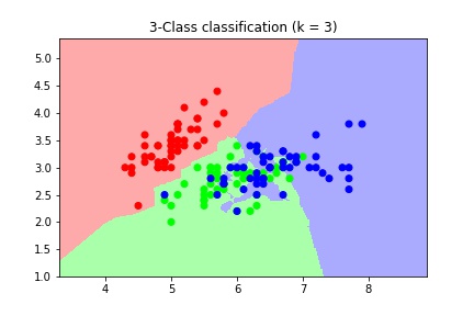

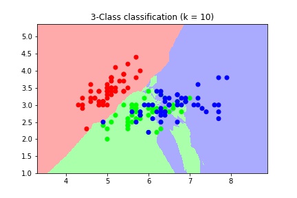
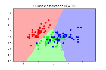
Decision boundary for different values of n_neighbors

As we can see, as the value of k increases, the decision boundary gets smoother. Therefore, we consider it to be a less complex model than those with lower k. Models with lower values of k are generally sensitive to noise present in the data and deviate from the required trends.

Classification is a very vast topic and perhaps the most applied one in the field of machine learning. The aim of the article was to introduce you to the topic and give you hands-on experience. Hopefully, you now have an idea about how classification works and have developed a basic understanding of the k-nearest neighbor algorithm. To gain further insight, refer to the following links:

• Kirril Fuchs’s article giving a brief description about commonly used classification algorithms
• Analytics Vidhya’s article on handling imbalanced classification.